
Objective and purpose
Image classifiers used under compute and latency constraints must balance predictive quality with resource use. Accuracy alone cannot establish which architecture fits a workload: a model can be more accurate on clean inputs yet perform worse on calibration, corruption response, or runtime. The objective is to compare a residual CNN and a Vision Transformer under matched parameter and estimated compute budgets, then evaluate how these tradeoffs affect model selection.
Model architectures and resource budgets
The completed experiment compares two custom PyTorch implementations on CIFAR-100: a residual convolutional network and a compact Vision Transformer. The implementation includes the models and attention blocks, training and evaluation pipelines, provenance checks, aggregation, and the selector. The study contains six full runs: both architectures at seeds 11, 29, and 47.
Matching parameter counts and estimated compute controls two sources of variation without isolating architecture as the sole cause of measured differences. The models also differ in normalization, initialization, and dropout. The experiment therefore compares two implementations under a shared evaluation and optimization protocol.
The CNN processes local image neighborhoods with convolutions. Residual connections add each block’s transformation to its shortcut representation. The ViT divides the image into patches and uses self-attention to mix information across those patches.
| Property | Residual CNN | Compact ViT |
|---|---|---|
| Input | 32 × 32 RGB image | 32 × 32 RGB image |
| Main structure | 7 residual blocks; widths 24, 48, 96, 192 | 7 Transformer blocks; width 128; 4 attention heads |
| Representation | Convolutions downsample 32 → 16 → 8 → 4 | 64 patches of 4 × 4 pixels, plus a class token |
| Classifier | Global spatial mean → 100 classes | Normalized class token → 100 classes |
| Parameters | 959,452 | 955,236 |
| Forward MACs per image | 67,922,688 | 67,614,976 |
| Normalization / dropout | Batch normalization / 0 | Layer normalization / 0.10 |
The CNN begins with a 3 × 3 convolution and uses stage depths of 1, 3, 2, and 1 blocks. Each residual block contains two 3 × 3 convolutions. Downsampling blocks use a projected shortcut. The architecture is a custom compact residual network rather than a standard ResNet-18.
The ViT uses learned patch embeddings, a class token, and positional embeddings. Each block applies normalization before attention and before its two-layer MLP, which expands from 128 to 256 features and returns to 128 through a GELU activation. Query, key, and value projections and attention operations are implemented explicitly.
Parameter counts differ by about 0.44%; estimated forward multiply–accumulate operations differ by about 0.45%. The training-compute estimate is approximately 1.83 × 10¹⁵ FLOPs per run. The estimate derives from forward MACs and processed example counts, excludes operations such as normalization and softmax, and does not measure executed accelerator operations.
Training and evaluation protocol
- 01Fixed dataset split45,000 training images, 5,000 validation images, and the official 10,000-image test set.
- 02Paired-seed training100 epochs per run, random initialization, and the same optimizer and augmentation recipe.
- 03Evaluation and aggregationClean and corrupted inputs, probability quality, runtime, and three-seed variation.
CIFAR-100 contains 100 fine-grained classes grouped into 20 coarse categories. A stratified split with seed 4771 partitions the official 50,000 training images. Training uses random 32-pixel crops with four pixels of padding, horizontal flips, and fixed channel normalization. Evaluation only normalizes the images. Channel means are (0.5071, 0.4867, 0.4408), with standard deviations (0.2675, 0.2565, 0.2761). Evaluation uses batches of 256.
Both models train for 100 epochs with AdamW, a learning rate of 0.0003, weight decay of 0.05, and batches of 128. A five-epoch warmup precedes per-batch cosine decay. Mixed precision and gradient clipping at 1 are enabled. The recipe uses no label smoothing or early stopping. Each run processes 4.5 million training examples over 35,200 optimizer steps.
The checkpoint with the highest validation top-1 accuracy supplies final test measurements; ties keep the earlier checkpoint. Selected epochs range from 76 to 100 for the CNN and 81 to 98 for the ViT. Checkpoint selection does not use test accuracy.
Gaussian-noise evaluation
The noise condition adds Gaussian noise with standard deviation 0.15 to pixel values on a 0–1 scale, clips them back into that range, and reapplies normalization. Both models receive the same deterministic corruption for each test image. This evaluates one corruption family at one severity. It is not the CIFAR-100-C benchmark.
Runtime measurement protocol
Runs use the Tesla T4 hardware profile with PyTorch 2.11.0, CUDA 12.8, and mixed precision. Single-image timing uses 10 warmups and 50 synchronized measurements on a prepared test image. It includes the CPU-to-GPU copy, input adaptation, and forward pass; it excludes decoding and CPU image transforms. These measurements describe this execution path, not a deployed serving system.
Predictive quality, corruption response, and efficiency
Higher CNN accuracy on clean images
The CNN achieves a 5.34 percentage-point accuracy advantage under the shared training protocol.
Custom models with approximately 1M parameters · CIFAR-100 · Random initialization · Three-seed means
Aggregate metric table
| Metric | CNN | ViT |
|---|---|---|
| Clean accuracy (%) | 60.96 | 55.62 |
| Noise accuracy (%) | 5.03 | 12.90 |
| Latency (ms) | 3.142 | 10.495 |
| Calibration (ECE) | 0.1354 | 0.1179 |
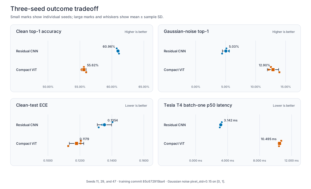
The CNN leads clean top-1 accuracy by 5.34 percentage points. Under noise, the ViT leads by 7.87 points, but both lose most of their clean accuracy. The relative ranking does not capture the substantial absolute accuracy loss in both models.
| Metric | CNN | ViT |
|---|---|---|
| Top-1 accuracy ↑ | 60.96% ± 0.18 pp | 55.62% ± 0.37 pp |
| Top-5 accuracy ↑ | 86.51% ± 0.16 pp | 82.92% ± 0.27 pp |
| Negative log-likelihood ↓ | 1.5960 ± 0.0228 | 1.7805 ± 0.0154 |
| Expected calibration error ↓ | 0.1354 ± 0.0045 | 0.1179 ± 0.0045 |
| Brier score ↓ | 0.5392 ± 0.0020 | 0.5942 ± 0.0046 |
| Worst-class accuracy ↑ | 26.67% ± 3.79 pp | 22.67% ± 3.21 pp |
Expected calibration error (ECE) groups predictions into 15 confidence bins and measures the weighted gap between confidence and accuracy. Negative log-likelihood penalizes low probability on the true class. The multiclass Brier score measures squared probability error. Lower ECE alone does not establish better probability estimates by every criterion: clean NLL and Brier results favor the CNN.
| Metric | CNN | ViT |
|---|---|---|
| Top-1 accuracy ↑ | 5.03% ± 0.58 pp | 12.90% ± 0.94 pp |
| Top-5 accuracy ↑ | 14.90% ± 1.62 pp | 32.63% ± 1.51 pp |
| Negative log-likelihood ↓ | 11.0800 ± 0.7930 | 5.5301 ± 0.1822 |
| Expected calibration error ↓ | 0.6107 ± 0.0657 | 0.3760 ± 0.0151 |
| Brier score ↓ | 1.4478 ± 0.0815 | 1.1427 ± 0.0208 |
Per-class results quantify the extent of corruption failures. Across the three seeds, the CNN has zero accuracy in 62, 55, and 74 of the 100 classes under noise. The ViT has 22, 24, and 21 such classes. The project records per-class accuracy, but it does not include a saved gallery of individual failure images.
| Metric | CNN | ViT |
|---|---|---|
| Batch-one p50 latency ↓ | 3.142 ± 0.123 ms | 10.495 ± 0.189 ms |
| Batch-one p95 latency ↓ | 4.670 ± 1.304 ms | 14.091 ± 1.842 ms |
| Training examples / second ↑ | 1,573 ± 89 | 1,156 ± 51 |
| Training-only time ↓ | 2,866 ± 159 s | 3,896 ± 168 s |
Scroll across to read all columns.
| Model / seed | Selected epoch | Clean top-1 | Noise top-1 | p50 latency |
|---|---|---|---|---|
| CNN / 11 | 100 | 60.76% | 5.13% | 3.266 ms |
| CNN / 29 | 88 | 61.00% | 5.55% | 3.140 ms |
| CNN / 47 | 76 | 61.11% | 4.41% | 3.021 ms |
| ViT / 11 | 96 | 55.62% | 12.56% | 10.708 ms |
| ViT / 29 | 98 | 55.25% | 12.18% | 10.348 ms |
| ViT / 47 | 81 | 55.98% | 13.97% | 10.429 ms |
Training throughput excludes validation and final evaluation. Latency values average each run’s measured percentile; they are not percentiles computed over one pooled collection. Hardware profile matching improves comparability without guaranteeing an identical physical machine or session.
Selection rule and score decomposition
The selector is a deterministic weighted rule. It first applies eligibility constraints, including a 1.1-million-parameter ceiling in this report. Both models pass. It then combines clean accuracy (45%), noise accuracy (20%), one minus ECE (15%), relative latency (10%), and relative parameter efficiency (10%). No hard latency ceiling applies here.
Relative latency is the fastest candidate’s latency divided by each candidate’s latency. Parameter efficiency uses the same ratio with the smallest parameter count. Accuracy values enter as fractions. The resulting score is a preference score, not a probability of success.
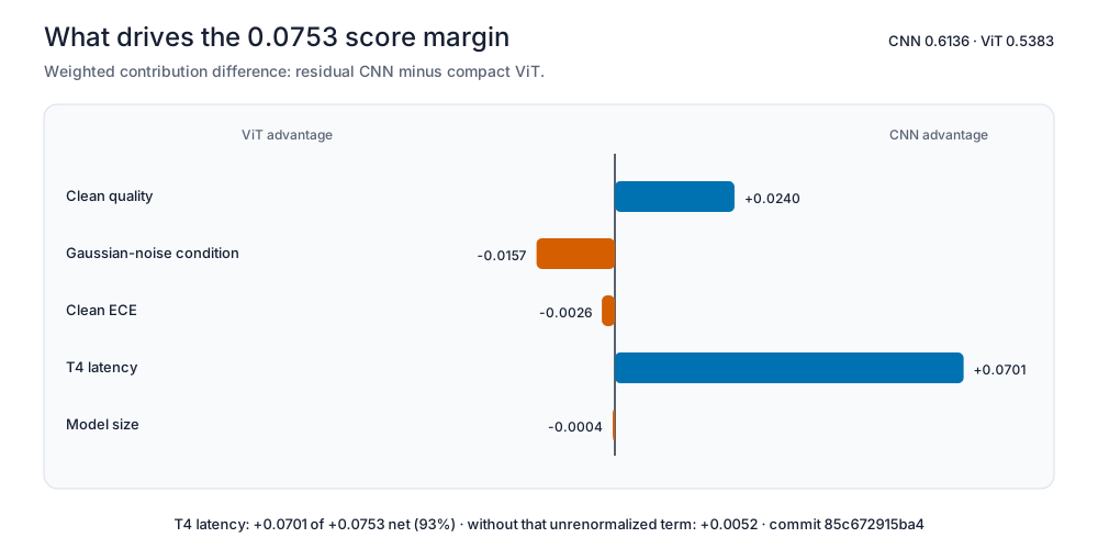
The final scores are 0.6136 for the CNN and 0.5383 for the ViT. Latency contributes about 0.0701 of the 0.0753 margin—roughly 93%. Removing latency leaves the CNN only slightly ahead, by about 0.0052 before rescaling the remaining weights.
The recommendation follows from these priorities and this hardware. A workload that places more value on the tested noise condition can justify a different choice. The component scores expose the recommendation’s dependence on the declared priorities.
Reproducibility controls and study limitations
The training system saves optimizer, scheduler, mixed-precision scaler, random-number state, history, and best-model weights so interrupted runs can resume. Checksum-verified exports and attempt-specific completion records reduce the chance of aggregating stale or partial runs.
Aggregation checks require the expected seeds and reject truncated smoke runs, inconsistent source provenance, and mismatched splits or preprocessing. Runtime comparisons require compatible hardware profiles. These checks reduce the risk of aggregating incompatible experiments.
Three seeds characterize run-to-run variation within this study but do not supply a formal significance analysis. One shared recipe may favor one implementation, and matched budgets do not remove dropout, normalization, and initialization differences. Peak-memory counters reset after resumed sessions, so existing memory records do not support a fair full-training memory ranking.
A transfer-learning arm is configured but has no completed study results. Broader corruption families, additional budgets, tuned recipes, and deployment measurements are also open work. The completed finding is a conditional recommendation for these two scratch-trained models.
Source code, measurements, and reproduction
The repository contains the implementation and reproduction instructions. Saved measurements, the decision report, and the training configuration provide the evidence behind this brief. No new model training was needed to reproduce the selector’s decision or verify the figures.
- Full measurement summary — per-seed metrics, aggregates, and experiment provenance.
- Selector decision and score components — the machine-readable recommendation.
- Scratch-training configuration — architecture and optimization settings.
After installing the repository package, use the measured-input configuration to validate the saved inputs and reproduce the decision without retraining:
vision-model-selector validate --config reports/cifar100-random-init-measured.toml
vision-model-selector recommend --config reports/cifar100-random-init-measured.toml --format markdown --output /tmp/cifar100-decision.md
Evidence: saved CIFAR-100 random-initialization reports and the project’s figure generator. Recorded training source commit: 85c672915ba495340a4df0713c55fdd7647001c3. Full training checkpoints are not bundled with this page.