
Objective and purpose
The objective is to evaluate whether trained linear autoencoders recover PCA’s principal subspace on MNIST, and how architecture and optimization affect that recovery. Reconstruction error alone cannot establish whether the methods learn equivalent subspaces.
Principal component analysis (PCA) and a linear autoencoder can both compress an image into a smaller representation and reconstruct the original pixels. PCA computes its principal subspace through linear algebra. An autoencoder learns an encoder and decoder through training. Their related reconstruction objectives motivate an empirical comparison of the learned autoencoder subspace with PCA’s principal subspace.
The MNIST experiments evaluate reconstruction error, principal angles, Grassmann distance, training behavior, and sensitivity to architecture and hyperparameters. These measurements distinguish reconstruction similarity from subspace alignment. The report also discusses downstream digit classification.
Research goals and theoretical background, pp. 2–5Model implementations and experimental conditions
The bottleneck imposes a rank constraint: mapping 784 pixel values into k latent coordinates restricts the linear reconstruction map to rank at most k. PCA identifies directions of maximum retained variance; a linear autoencoder optimizes encoder and decoder weights to minimize reconstruction loss. Finite optimization can terminate before reaching an optimum. Different weight matrices can also represent the same subspace, so the evaluation compares subspaces rather than requiring identical weights.
The NumPy PCA implementation centers the data, constructs the covariance matrix, computes its eigenvectors, and retains the leading components. The PyTorch autoencoder uses two fully connected layers, from 784 input features to k latent dimensions and back to 784. The network omits nonlinear activations, restricting the comparison to linear dimensionality reduction.
MNIST supplies 28 × 28 grayscale images. Preprocessing flattens each image into 784 features and normalizes pixel values to [0, 1]. The detailed training procedure uses the same mean-centered inputs for both methods, adding the mean back for image reconstruction. The reported result tables cover k = 8, 32, 64, and 128.
- Experiment 1: Unconstrained architecture. Independent encoder and decoder weights, with bias terms. A 10,000-image training subset, Adam, batch size 128, learning rate 0.001, and 50 epochs.
- Experiment 2: Constrained architecture. The same 10,000-image subset and baseline training budget. The decoder weights are tied to the encoder’s transpose, and both layers omit bias terms.
- Experiment 3: Optimization search. The constrained model on all 70,000 MNIST images, with different epoch budgets, initialization strategies, and learning-rate schedules. This experiment combines the official training and test sets to study full-dataset alignment.
Reconstruction error comparison
Mean squared error (MSE) averages the squared differences between reconstructed and original pixel values. Lower error means a closer reconstruction. Increasing k increases the permitted reconstruction rank; the reported reconstruction errors decrease with latent dimensionality.
The unconstrained autoencoder reconstructs the digits almost as well as PCA. Across the four latent sizes in Table 1, the report gives relative MSE differences below 4%. At k = 64, for example, PCA has an MSE of 0.0094 and the autoencoder has an MSE of 0.0095.
| Latent dimensions | PCA MSE | Autoencoder MSE |
|---|---|---|
| 8 | 0.0381 | 0.0385 |
| 32 | 0.0173 | 0.0174 |
| 64 | 0.0094 | 0.0095 |
| 128 | 0.0044 | 0.0045 |
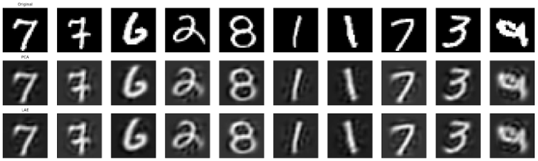
The constrained model also produces close reconstruction errors, with reported differences of 0.6%–3.4%. The paper describes similar downstream classification accuracy for the two methods: approximately 77% at k = 8 and 90% at k = 128. Those classification figures are supporting observations; the report does not give a complete classifier and evaluation-split specification.
Reconstruction and classification assess information retention and task utility. Subspace measurements separately assess geometric agreement with PCA.
Geometric alignment of learned subspaces
The geometric comparison measures alignment between the row space of the encoder weights and PCA’s principal subspace. Principal angles range from 0° for aligned directions to 90° for orthogonal directions. Mean and maximum angles characterize both average alignment and residual discrepancies. Grassmann distance summarizes the principal-angle vector in a scalar measure of separation.
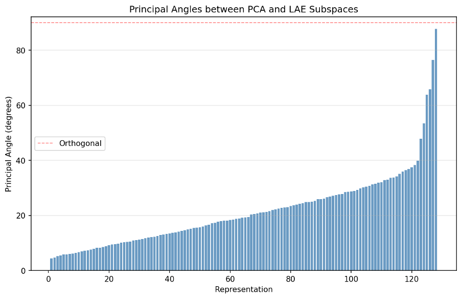
In Experiment 1, mean principal angles range from 21.5° to 49.6°, despite the close reconstruction errors. At k = 128, the mean is 21.5° and the largest angle is 87.7°. The unconstrained model therefore learns a representation that performs similarly on reconstruction while differing substantially from PCA under the geometric comparison.
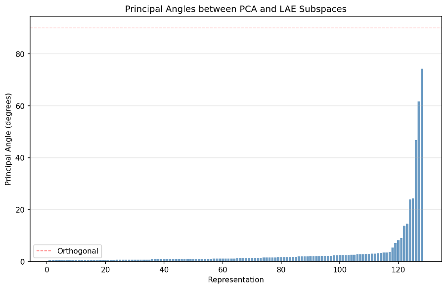
Experiment 2 changes two architectural choices together: it ties the weights and removes biases. Mean angles fall to 2.7°–4.5°, compared with 21.5°–49.6° in Experiment 1. The report gives a 6–11-fold improvement in mean alignment. Grassmann distances also fall, from 2.50–5.03 to 0.42–2.04.
Reported subspace alignment
Mean principal angle relative to PCA. Lower values indicate closer subspace alignment.
Experiment 1
Untied weights, with bias
10,000 images · 50 epochs
Experiment 2
Tied weights, no bias
10,000 images · 50 epochs
Experiment 3 · Best reported run
Tied weights, no bias
70,000 images · 200 epochs
Cosine schedule · Run 48
Experiment 3 changes both dataset size and training configuration. Reported values represent selected best runs. They do not provide averages across random seeds or isolate the effect of additional data.
View mean angles for all latent dimensions
| k | Experiment 1 | Experiment 2 | Experiment 3 Best run |
|---|---|---|---|
| 8 | 49.6° | 4.5° | 6.36° |
| 32 | 30.4° | 2.7° | 0.28° |
| 64 | 25.2° | 2.9° | 0.16° |
| 128 | 21.5° | 3.5° | 0.12° |
These experiments establish an observed improvement from the combined architectural change. They do not isolate the effect of weight tying from the effect of removing bias. Comparing subspaces also differs from comparing individual basis vectors: a change of basis within the same subspace does not by itself create nonzero principal angles.
Architecture comparison, Table 2 and Figure 3, p. 12Optimization sensitivity and best-run alignment
Experiment 3 evaluates residual alignment error for the constrained model on the full 70,000-image dataset. The configurations vary training duration, default versus orthogonal initialization, and constant versus cosine learning-rate schedules.
The best reported run at k = 128 reaches a mean principal angle of 0.12° with 200 epochs, orthogonal initialization, and cosine scheduling. The corresponding best means are 0.16° at k = 64 and 0.28° at k = 32. The result at the smallest latent dimensionality differs: the best reported k = 8 run reaches 6.36°, using 50 epochs and default initialization.
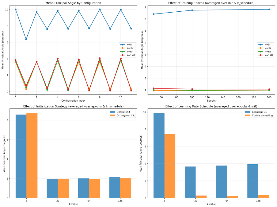
Learning-rate scheduling shows the largest separation in the summary figure. At k ≥ 32, cosine scheduling produces smaller mean principal angles than a constant rate. Default and orthogonal initialization produce similar averages, indicating a smaller observed effect than scheduling within the tested configurations.
The report also examines learning-rate magnitude, batch size, and random-seed variation. These comparisons show that a shared reconstruction objective does not eliminate optimization sensitivity. The reported 0.12° is the mean principal angle of a selected best run, not an average across repeated runs or a guarantee for another dataset.
Best configurations and hyperparameter analysis, Table 3 and pp. 13–15Interpretation and methodological limitations
The tested MNIST configurations produce similar reconstruction quality. Recovery of PCA’s principal subspace requires a separate geometric assessment because reconstruction error alone does not establish alignment.
For the tested constrained models, cosine scheduling and the selected training budgets produce substantially lower mean angles at larger latent dimensionalities. These results support direct evaluation of subspace alignment alongside reconstruction error and explicit measurement of architectural and optimization effects.
Limitations and future experiments
- Constraint isolation. Weight tying and bias removal change together. The paper proposes testing their effects independently.
- Convergence and generalization. Experiment 3 combines MNIST’s official training and test sets. Its results concern full-dataset subspace alignment, not performance on unseen digits.
- Confounded experimental changes. Dataset size and training choices both change in Experiment 3. The results do not isolate the effect of adding more data, and the best k = 8 result does not improve on Experiment 2.
- Dataset and eigenspectrum coverage. The study uses one dataset, a limited search, and no complete analysis of the eigenspectrum. The paper proposes broader datasets and nonlinear autoencoders as future work.
Basis dependence and subspace invariance
The interactive illustration demonstrates basis rotation and subspace inclination. Its values are illustrative; the preceding sections report the experimental measurements.
Basis rotation and subspace alignment
Synthetic geometric illustration. Displayed values describe the selected transformation rather than measurements from the research report.
- Largest principal angle
- 0°
- Projector distance (Frobenius)
- 0.000
Rotation within the plane changes the basis and preserves the spanned subspace. Individual vector comparisons can therefore differ from subspace comparisons.
Contribution
My contributions included refining the PCA and autoencoder code for comparable latent representations, adding principal-angle and Grassmann-distance metrics, and helping structure experiments around architecture, latent dimensionality, and training hyperparameters. I also contributed to the paper’s structure and organization. The implementation, experiments, and report reflect the work of all five coauthors.
Paper and implementation resources
The full report contains the mathematical background, experimental setup, result tables, figures, discussion, and bibliography. The shared repository contains the PCA and autoencoder implementations and the saved experiment outputs.
All reported values and four figures come from the final report dated December 15, 2025. The figures retain the paper’s original data and labels.